
7 Linear Motion

Figure 7.1 These cyclists in Vietnam can be described by their position relative to buildings and a canal. Their motion can be described by their change in position, or displacement, in the frame of reference. (credit: Suzan Black, Fotopedia)
Position
In order to describe the motion of an object, you must first be able to describe its position—where it is at any particular time. More precisely, you need to specify its position relative to a convenient reference frame. Earth is often used as a reference frame, and we often describe the position of an object as it relates to stationary objects in that reference frame. For example, a rocket launch would be described in terms of the position of the rocket with respect to the Earth as a whole, while a professor’s position could be described in terms of where she is in relation to the nearby white board. (See Figure 7.2) In other cases, we use reference frames that are not stationary but are in motion relative to the Earth. To describe the position of a person in an airplane, for example, we use the airplane, not the Earth, as the reference frame. (See Figure 7.3)
Displacement
If an object moves relative to a reference frame (for example, if a professor moves to the right relative to a white board or a passenger moves toward the rear of an airplane), then the object’s position changes. This change in position is known as displacement. The word “displacement” implies that an object has moved, or has been displaced.
Displacement is the change in position of an object: Δx = xf−x0, where xf is the final position, and x0 is the initial position.
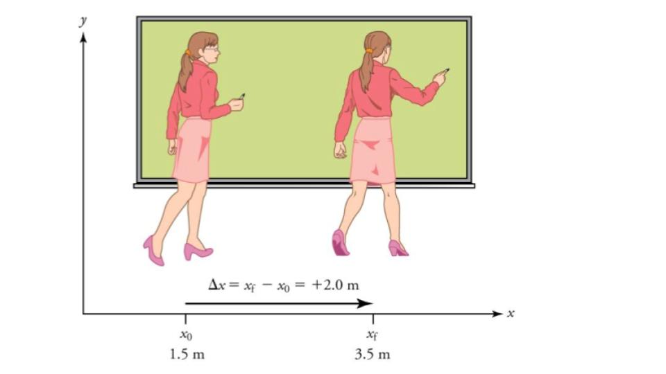 Figure 7.2 A professor paces left and right while lecturing. Her position relative to Earth is given by x. The +2.0m displacement of the professor relative to Earth is represented by an arrow pointing to the right.
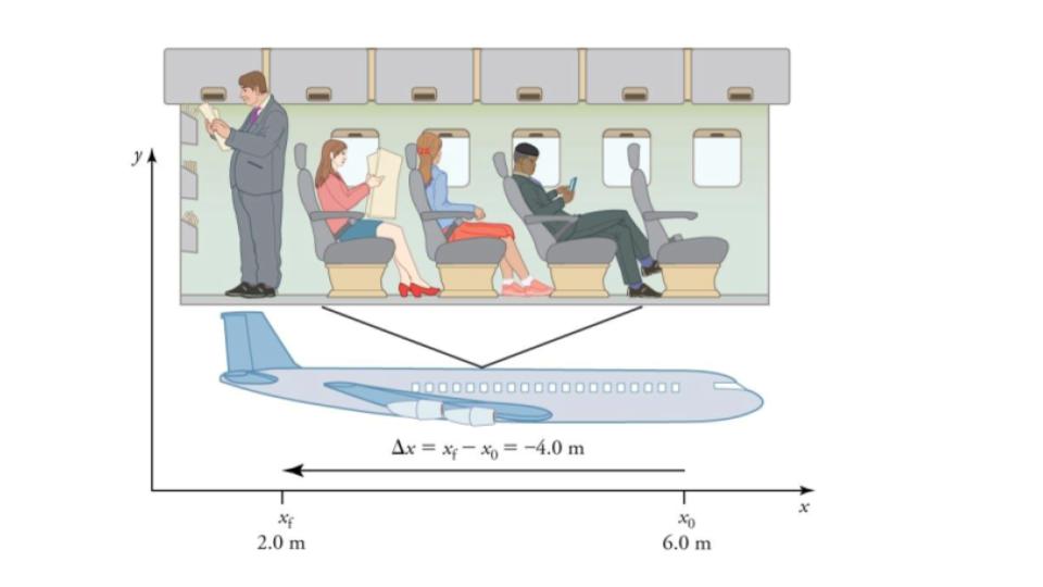
Figure 7.3 A passenger moves from his seat to the back of the plane. His location relative to the airplane is given by x. The −4.0m displacement of the passenger relative to the plane is represented by an arrow toward the rear of the plane. Notice that the arrow representing his displacement is twice as long as the arrow representing the displacement of the professor (he moves twice as far) in Figure 7.2.
Note that displacement has a direction as well as a magnitude. The professor’s displacement is 2.0 m to the right, and the airline passenger’s displacement is 4.0 m toward the rear. In one-dimensional motion, direction can be specified with a plus or minus sign. When you begin a problem, you should select which direction is positive (usually that will be to the right or up, but you are free to select positive as being any direction). The professor’s initial position is x0 = 1.5m and her final position is xf = 3.5m. Thus her displacement is Δx = xf−x0 = 3.5 m−1.5 m = +2.0 m.
In this coordinate system, motion to the right is positive, whereas motion to the left is negative. Similarly, the airplane passenger’s initial position is x0 = 6.0 m and his final position is xf = 2.0 m.
Δx = xf−x0 = 2.0 m−6.0 m = −4.0 m.
His displacement is negative because his motion is toward the rear of the plane, or in the negative direction in our coordinate system.
Distance
Although displacement is described in terms of direction, distance is not. Distance is defined to be the magnitude or size of displacement between two positions. Note that the distance between two positions is not the same as the distance traveled between them. Distance traveled is the total length of the path traveled between two positions. Distance has no direction and, thus, no sign. For example, the distance the professor walks is 2.0 m. The distance the airplane passenger walks is 4.0 m.
MISCONCEPTION ALERT: DISTANCE TRAVELED VS. MAGNITUDE OF DISPLACEMENT
It is important to note that the distance traveled, however, can be greater than the magnitude of the displacement (by magnitude, we mean just the size of the displacement without regard to its direction; that is, just a number with a unit). For example, the professor could pace back and forth many times, perhaps walking a distance of 150 m during a lecture, yet still end up only 2.0 m to the right of her starting point. In this case her displacement would be +2.0 m, the magnitude of her displacement would be 2.0 m, but the distance she traveled would be 150 m. In kinematics we nearly always deal with displacement and magnitude of displacement, and almost never with distance traveled. One way to think about this is to assume you marked the start of the motion and the end of the motion. The displacement is simply the difference in the position of the two marks and is independent of the path taken in traveling between the two marks. The distance traveled, however, is the total length of the path taken between the two marks.

Figure 7.4 The motion of these racing snails can be described by their speeds and their velocities. (credit: tobitasflickr, Flickr)
There is more to motion than distance and displacement. Questions such as, “How long does a foot race take?” and “What was the runner’s speed?” cannot be answered without an understanding of other concepts. In this section we add definitions of time, velocity, and speed to expand our description of motion.
Time
As discussed in Chapter 1, Measurements, the most fundamental physical quantities are defined by how they are measured. This is the case with time. Every measurement of time involves measuring a change in some physical quantity. It may be a number on a digital clock, a heartbeat, or the position of the Sun in the sky. In physics, the definition of time is simple—time is change, or the interval over which change occurs. It is impossible to know that time has passed unless something changes.
The amount of time or change is calibrated by comparison with a standard. The SI unit for time is the second (s). We might, for example, observe that a certain pendulum makes one full swing every 0.75 s. We could then use the pendulum to measure time by counting its swings or by connecting the pendulum to a clock mechanism that registers time on a dial. This allows us to not only measure the amount of time, but also to determine a sequence of events.
How does time relate to motion? We are usually interested in elapsed time for a particular motion, such as how long it takes an airplane passenger to get from his seat to the back of the plane. To find elapsed time, we note the time at the beginning and end of the motion and subtract the two. For example, a lecture may start at 11:00 A.M. and end at 11:50 A.M., so that the elapsed time would be 50 min. Elapsed time Δt is the difference between the ending time and beginning time,
Δt = tf−t0, where Δt is the change in time or elapsed time, tf is the time at the end of the motion, and t0 is the time at the beginning of the motion. (As usual, the delta symbol, Δ, means the change in the quantity that follows it.)
Life is simpler if the beginning time t0 is taken to be zero, as when we use a stopwatch. If we were using a stopwatch, it would simply read zero at the start of the lecture and 50 min at the end. If t0 = 0, then Δt = tf ≡ t.
Velocity
Your notion of velocity is probably the same as its scientific definition. You know that if you have a large displacement in a small amount of time you have a large velocity, and that velocity has units of distance divided by time, such as miles per hour or kilometers per hour.
Average Velocity
Average velocity is displacement (change in position) divided by the time of travel,
average v = Δx/Δt
Notice that this definition indicates that velocity is a vector because displacement is a vector. It has both magnitude and direction. The SI unit for velocity is meters per second or m/s, but many other units, such as km/h, mi/h (also written as mph), and cm/s, are in common use. Suppose, for example, an airplane passenger took 5 seconds to move −4 m (the negative sign indicates that displacement is toward the back of the plane). His average velocity would be:
average v = Δx/Δt = −4m / 5s = −0.8 m/s.
The minus sign indicates the average velocity is also toward the rear of the plane.
The average velocity of an object does not tell us anything about what happens to it between the starting point and ending point, however. For example, we cannot tell from average velocity whether the airplane passenger stops momentarily or backs up before he goes to the back of the plane. To get more details, we must consider smaller segments of the trip over smaller time intervals.
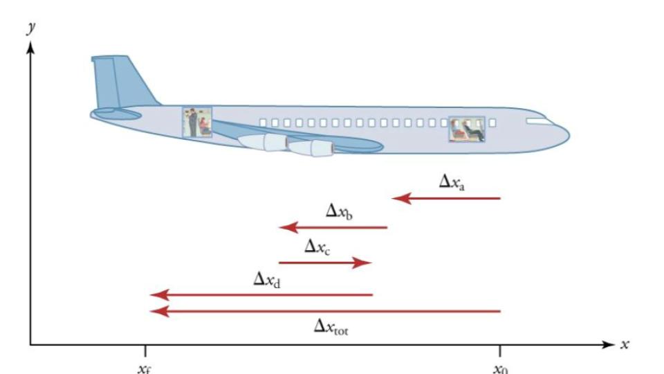
Figure 7.5 A more detailed record of an airplane passenger heading toward the back of the plane, showing smaller segments of his trip.
The smaller the time intervals considered in a motion, the more detailed the information. When we carry this process to its logical conclusion, we are left with an infinitesimally small interval. Over such an interval, the average velocity becomes the instantaneous velocity or the velocity at a specific instant. A car’s speedometer, for example, shows the magnitude (but not the direction) of the instantaneous velocity of the car. (Police give tickets based on instantaneous velocity, but when calculating how long it will take to get from one place to another on a road trip, you need to use average velocity.)
Speed
In everyday language, most people use the terms “speed” and “velocity” interchangeably. In physics, however, they do not have the same meaning and they are distinct concepts. One major difference is that speed has no direction. Thus speed is a scalar. Just as we need to distinguish between instantaneous velocity and average velocity, we also need to distinguish between instantaneous speed and average speed.
Instantaneous speed is the magnitude of instantaneous velocity. For example, suppose the airplane passenger at one instant had an instantaneous velocity of −3.0 m/s (the minus meaning toward the rear of the plane). At that same time his instantaneous speed was 3.0 m/s. Or suppose that at one time during a shopping trip your instantaneous velocity is 40 km/h due north. Your instantaneous speed at that instant would be 40 km/h—the same magnitude but without a direction. Average speed, however, is very different from average velocity. Average speed is the distance traveled divided by elapsed time.
We have noted that distance traveled can be greater than the magnitude of displacement. So average speed can be greater than average velocity, which is displacement divided by time. For example, if you drive to a store and return home in half an hour, and your car’s odometer shows the total distance traveled was 6 km, then your average speed was 12 km/h. Your average velocity, however, was zero, because your displacement for the round trip is zero. (Displacement is change in position, and thus, is zero for a round trip.) Thus average speed is not simply the magnitude of average velocity.
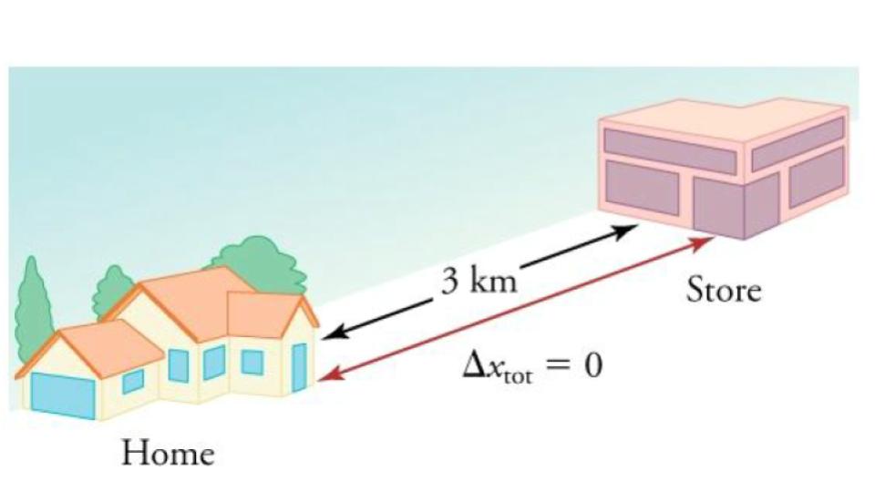
Figure 7.6 During a 30-minute round trip to the store, the total distance traveled is 6 km. The average speed is 12 km/h. The displacement for the round trip is zero, since there was no net change in position. Thus the average velocity is zero.
Another way of visualizing the motion of an object is to use a graph. A plot of position or of velocity as a function of time can be very useful. For example, for this trip to the store, the position, velocity, and speed-vs.-time graphs are displayed in Figure 7.7. (Note that these graphs depict a very simplified model of the trip. We are assuming that speed is constant during the trip, which is unrealistic given that we’ll probably stop at the store. But for simplicity’s sake, we will model it with no stops or changes in speed. We are also assuming that the route between the store and the house is a perfectly straight line.)
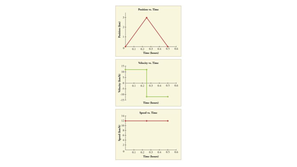
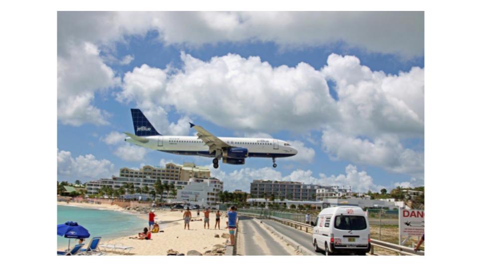
Figure 7.8 A plane decelerates, or slows down, as it comes in for landing in St. Maarten. Its acceleration is opposite in direction to its velocity. (credit: Steve Conry, Flickr)
In everyday conversation, to accelerate means to speed up. The accelerator in a car can in fact cause it to speed up. The greater the acceleration, the greater the change in velocity over a given time. The formal definition of acceleration is consistent with these notions, but more inclusive.
Average Acceleration
Average Acceleration is the rate at which velocity changes,
average a = Δv / Δt = (vf−v0) / (tf−t0),
Because acceleration is velocity in m/s divided by time in s, the SI units for acceleration are meters per second squared or meters per second per second, which literally means by how many meters per second the velocity changes every second.
Recall that velocity is a vector—it has both magnitude and direction. This means that a change in velocity can be a change in magnitude (or speed), but it can also be a change in direction. For example, if a car turns a corner at constant speed, it is accelerating because its direction is changing. The quicker you turn, the greater the acceleration. So there is an acceleration when velocity changes either in magnitude (an increase or decrease in speed) or in direction, or both.
Acceleration as a Vector
Acceleration is a vector in the same direction as the change in velocity, Δv. Since velocity is a vector, it can change either in magnitude or in direction. Acceleration is therefore a change in either speed, direction, or both.
Keep in mind that although acceleration is in the direction of the change in velocity, it is not always in the direction of motion. When an object slows down, its acceleration is opposite to the direction of its motion. This is known as deceleration.
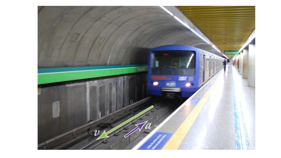
Figure 7.9 A subway train in Sao Paulo, Brazil, decelerates as it comes into a station. It is accelerating in a direction opposite to its direction of motion. (credit: Yusuke Kawasaki, Flickr)
MISCONCEPTION ALERT: DECELERATION VS. NEGATIVE ACCELERATION
Deceleration always refers to acceleration in the direction opposite to the direction of the velocity. Deceleration always reduces speed. Negative acceleration, however, is acceleration in the negative direction in the chosen coordinate system. Negative acceleration may or may not be deceleration, and deceleration may or may not be considered negative acceleration. For example, consider Figure 7.10.
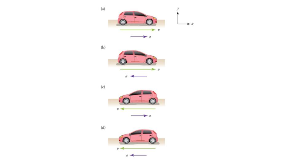
Figure 7.10 (a) This car is speeding up as it moves toward the right. It therefore has positive acceleration in our coordinate system. (b) This car is slowing down as it moves toward the right. Therefore, it has negative acceleration in our coordinate system, because its acceleration is toward the left. The car is also decelerating: the direction of its acceleration is opposite to its direction of motion. (c) This car is moving toward the left, but slowing down over time. Therefore, its acceleration is positive in our coordinate system because it is toward the right. However, the car is decelerating because its acceleration is opposite to its motion. (d) This car is speeding up as it moves toward the left. It has negative acceleration because it is accelerating toward the left. However, because its acceleration is in the same direction as its motion, it is speeding up (not decelerating).
EXAMPLE 7.1 CALCULATING ACCELERATION: A RACEHORSE LEAVES THE GATE
A racehorse coming out of the gate accelerates from rest to a velocity of 15.0 m/s due west in 1.80 s. What is its average acceleration?
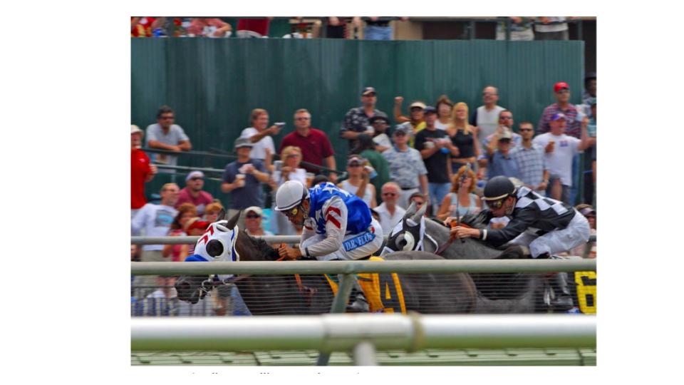
Figure 7.11 (credit: Jon Sullivan, PD Photo.org)
Strategy
First we draw a sketch and assign a coordinate system to the problem. This is a simple problem, but it always helps to visualize it. Notice that we assign east as positive and west as negative. Thus, in this case, we have negative velocity.
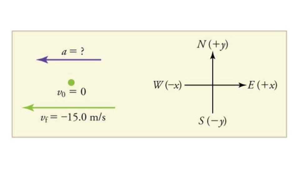
Figure 7.12
We can solve this problem by identifying Δv and Δt from the given information and then calculating the average acceleration directly from the equation a = Δv/Δt = (vf−v0) / (tf−t0).
Solution
- Identify the knowns. v0 = 0 m/s, vf = −15.0 m/s (the negative sign indicates direction toward the west), Δt = 1.80 s.
- Find the change in velocity. Since the horse is going from zero to −15.0 m/s, its change in velocity equals its final velocity: Δv= vf = −15.0 m/s.
- Plug in the known values (Δv and Δt) and solve for the unknown a.
average a = Δv/Δt = (−15.0 m/s) / (1.80 s) = −8.33 m/s2.
Discussion
The negative sign for acceleration indicates that acceleration is toward the west. An acceleration of 8.33 m/s2 due west means that the horse increases its velocity by 8.33 m/s due west each second, that is, 8.33 meters per second per second, which we write as 8.33 m/s2. This is truly an average acceleration, because the ride is not smooth. We shall see later that an acceleration of this magnitude would require the rider to hang on with a force nearly equal to his weight.
Instantaneous Acceleration
Instantaneous acceleration a, or the acceleration at a specific instant in time, is similar to instantaneous velocity —that is, considering an infinitely small interval of time. How do we find instantaneous acceleration using only algebra? The answer is that we choose an average acceleration that is representative of the motion. Figure 7.13 shows graphs of instantaneous acceleration versus time for two very different motions. In Figure 7.13(a), the acceleration varies slightly and the average over the entire interval is nearly the same as the instantaneous acceleration at any time. In this case, we should treat this motion as if it had a constant acceleration equal to the average (in this case about 1.8 m/s2). In Figure 7.13(b), the acceleration varies drastically over time. In such situations it is best to consider smaller time intervals and choose an average acceleration for each. For example, we could consider motion over the time intervals from 0 s to 1.0 s and from 1.0 s to 3.0 s as separate motions with accelerations of +3.0 m/s2 and –2.0 m/s2, respectively.
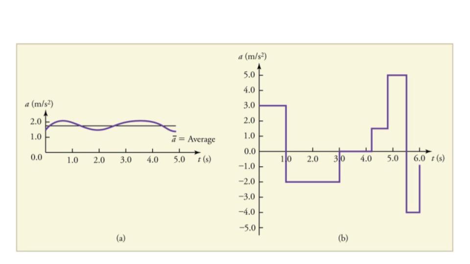
Figure 7.13 Graphs of instantaneous acceleration versus time for two different one-dimensional motions. (a) Here acceleration varies only slightly and is always in the same direction, since it is positive. The average over the interval is nearly the same as the acceleration at any given time. (b) Here the acceleration varies greatly, perhaps representing a package on a post office conveyor belt that is accelerated forward and backward as it bumps along. It is necessary to consider small time intervals (such as from 0 s to 1.0 s) with constant or nearly constant acceleration in such a situation.
The next several examples consider the motion of the subway train shown in Figure 7.14. In (a) the shuttle moves to the right, and in (b) it moves to the left. The examples are designed to further illustrate aspects of motion and to illustrate some of the reasoning that goes into solving problems.
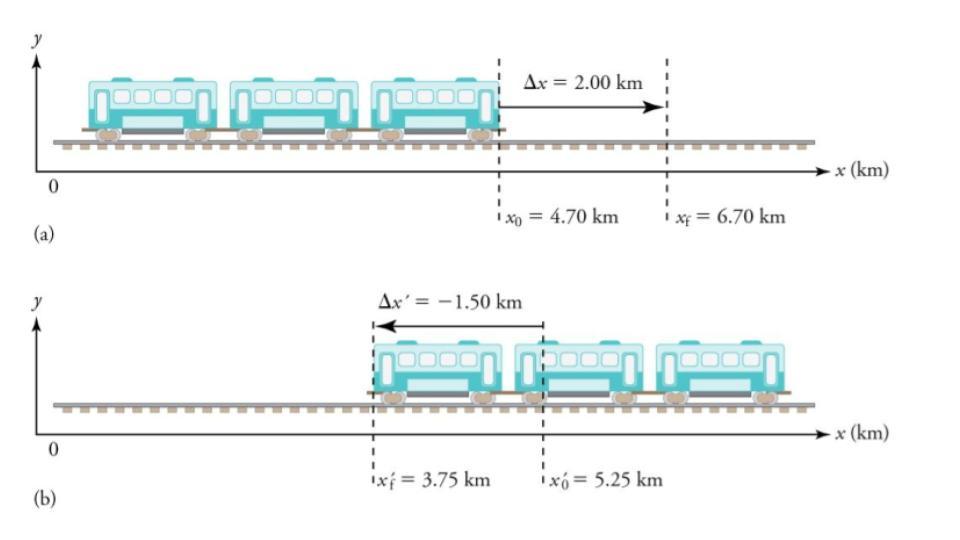
Figure 7.14 One-dimensional motion of a subway train considered in Example 7.2, Example 7.3, Example 7.4, Example 7.5. Here we have chosen the x-axis so that + means to the right and − means to the left for displacements, velocities, and accelerations. (a) The subway train moves to the right from x0 to xf. Its displacement Δx is +2.0 km. (b) The train moves to the left from x0‘ to xf‘. Its displacement Δx’ is −1.5 km. (Note that the prime symbol (′) is used simply to distinguish between displacement in the two different situations. The distances of travel and the size of the cars are on different scales to fit everything into the diagram.)
EXAMPLE 7.2 CALCULATING DISPLACEMENT: A SUBWAY TRAIN
What are the magnitude and sign of displacements for the motions of the subway train shown in parts (a) and (b) of Figure 7.14?
Strategy
A drawing with a coordinate system is already provided, so we don’t need to make a sketch, but we should analyze it to make sure we understand what it is showing. Pay particular attention to the coordinate system. To find displacement, we use the equation Δx = xf−x0. This is straightforward since the initial and final positions are given.
Solution
- Identify the knowns. In the figure we see that xf = 6.70 km and x0 = 4.70 km for part (a), and xf‘= 3.75 km and x0‘ = 5.25 km for part (b).
- Solve for displacement in part (a).
Δx = xf−x0 = 6.70 km−4.70 km = +2.00 km
- Solve for displacement in part (b).
Δx’ = xf‘−x0‘ = 3.75 km−5.25 km = −1.50 km
Discussion
The direction of the motion in (a) is to the right and therefore its displacement has a positive sign, whereas motion in (b) is to the left and thus has a negative sign.
EXAMPLE 7.3 COMPARING DISTANCE TRAVELED WITH DISPLACEMENT: A SUBWAY TRAIN
What are the distances traveled for the motions shown in parts (a) and (b) of the subway train in Figure 7.14?
Strategy
To answer this question, think about the definitions of distance and distance traveled, and how they are related to displacement. Distance between two positions is defined to be the magnitude of displacement, which was found in Example 7.2. Distance traveled is the total length of the path traveled between the two positions. In the case of the subway train shown in Figure 7.14, the distance traveled is the same as the distance between the initial and final positions of the train.
Solution
- The displacement for part (a) was +2.00 km. Therefore, the distance between the initial and final positions was 2.00 km, and the distance traveled was 2.00 km.
- The displacement for part (b) was −1.5 km. Therefore, the distance between the initial and final positions was 1.50 km, and the distance traveled was 1.50 km.
EXAMPLE 7.4 CALCULATING AVERAGE VELOCITY: THE SUBWAY TRAIN
What is the average velocity of the train in part b of Example 7.2 (and shown again below) if it takes 5.00 min to make its trip?
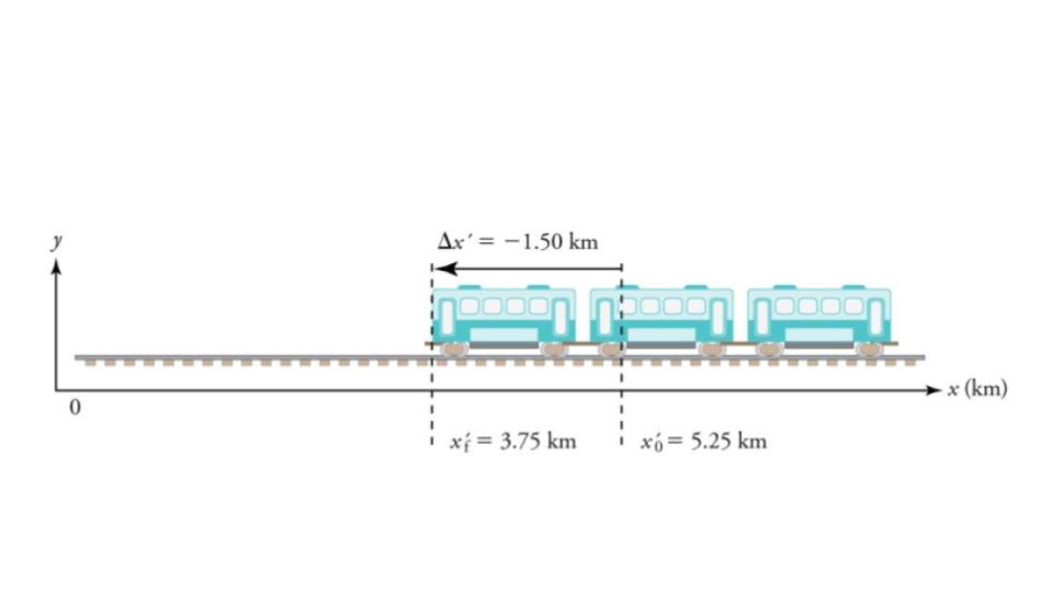
Figure 7.15
Strategy
Average velocity is displacement divided by time. It will be negative here, since the train moves to the left and has a negative displacement.
Solution
- Identify the knowns. xf‘ = 3.75 km, x0‘ = 5.25 km, Δt = 5.00 min.
- Determine displacement, Δx’. We found Δx’ to be −1.5 km in Example 7.2.
- Solve for average velocity.
average v = Δx’/Δt = (−1.50 km)/(5.00 min)
- Convert units.
average v = Δx’/Δt = ((−1.50 km)/(5.00 min)) * (60 min /1 h) = −18.0 km/h
Discussion
The negative velocity indicates motion to the left.
EXAMPLE 7.5 CALCULATING DECELERATION: THE SUBWAY TRAIN
Finally, suppose the train in Figure 7.15 slows to a stop from a velocity of 20.0 km/h in 10.0 s. What is its average acceleration?
Strategy
Once again, let’s draw a sketch:
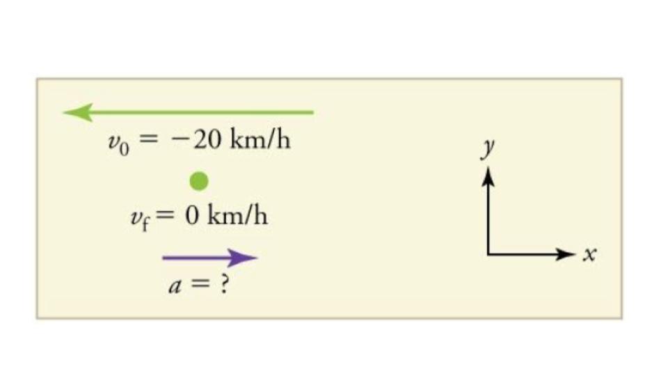
Figure 7.16
As before, we must find the change in velocity and the change in time to calculate average acceleration.
Solution
- Identify the knowns. v0 = −20 km/h, vf = 0 km/h, Δt = 10.0 s.
- Calculate Δv. The change in velocity here is actually positive, since Δv = vf−v0 = 0−(−20 km/h)=+20 km/h.
- Solve for acceleration.
a = Δv/Δt = (+20.0 km/h)/(10.0 s)
- Convert units.
a = ((+20.0 km/h)/(10.0 s)) * (103m/1 km) * (1 h/3600 s) = +0.556 m/s2
Discussion
The plus sign means that acceleration is to the right. This is reasonable because the train initially has a negative velocity (to the left) in this problem and a positive acceleration opposes the motion (and so it is to the right). Again, acceleration is in the same direction as the change in velocity, which is positive here. This acceleration can be called a deceleration since it is in the direction opposite to the velocity.

Figure 7.17 Kinematic equations can help us describe and predict the motion of moving objects such as these kayaks racing in Newbury, England. (credit: Barry Skeates, Flickr)
We might know that the greater the acceleration of, say, a car moving away from a stop sign, the greater the displacement in a given time. But we have not developed a specific equation that relates acceleration and displacement. In this section, we develop some convenient equations for kinematic relationships, starting from the definitions of displacement, velocity, and acceleration already covered.
Notation: t, x, v, a
First, let us make some simplifications in notation. Taking the initial time to be zero, as if time is measured with a stopwatch, is a great simplification. Since elapsed time is Δt = tf−t0, taking t0 = 0 means that Δt = tf, the final time on the stopwatch. When initial time is taken to be zero, we use the subscript 0 to denote initial values of position and velocity. That is, x0 is the initial position and v0 is the initial velocity. We put no subscripts on the final values. That is, t is the final time, x is the final position, and v is the final velocity. This gives a simpler expression for elapsed time—now, Δt = t. The expression for displacement is now Δx = x-x0, and the expression for change in velocity is now Δv = v−v0. We now make the important assumption that acceleration is constant. This assumption allows us to avoid using calculus to find instantaneous acceleration. Since acceleration is constant, the average and instantaneous accelerations are equal. That is, average a = a = constant, so we use the symbol a for acceleration at all times. Assuming acceleration to be constant does not seriously limit the situations we can study nor degrade the accuracy of our treatment. For one thing, acceleration is constant in a great number of situations. Furthermore, in many other situations we can accurately describe motion by assuming a constant acceleration equal to the average acceleration for that motion. Finally, in motions where acceleration changes drastically, such as a car accelerating to top speed and then braking to a stop, the motion can be considered in separate parts, each of which has its own constant acceleration.
SOLVING FOR DISPLACEMENT (Δx) AND FINAL POSITION (x) FROM AVERAGE VELOCITY WHEN ACCELERATION (a) IS CONSTANT
To get our first two new equations, we start with the definition of average velocity:
average v = Δx/Δt.
Substituting the simplified notation for Δx and Δt yields average v = (x−x0)/t.
Solving for x yields
x = x0+(average v)t,
where the average velocity is
average v = (v0+v)/2 (constant a)
The equation average v = (v0+v)/2 reflects the fact that, when acceleration is constant, average v is just the simple average of the initial and final velocities. For example, if you steadily increase your velocity (that is, with constant acceleration) from 30 to 60 km/h, then your average velocity during this steady increase is 45 km/h. Using the equation average v = (v0+v)/2 to check this, we see that
average v = (v0+v)/2 = (30 km/h+60 km/h)/2 = 45 km/h,
which seems logical.
EXAMPLE 7.6 CALCULATING DISPLACEMENT: HOW FAR DOES THE JOGGER RUN?
A jogger runs down a straight stretch of road with an average velocity of 4.00 m/s for 2.00 min. What is his final position, taking his initial position to be zero?
Strategy
Draw a sketch.
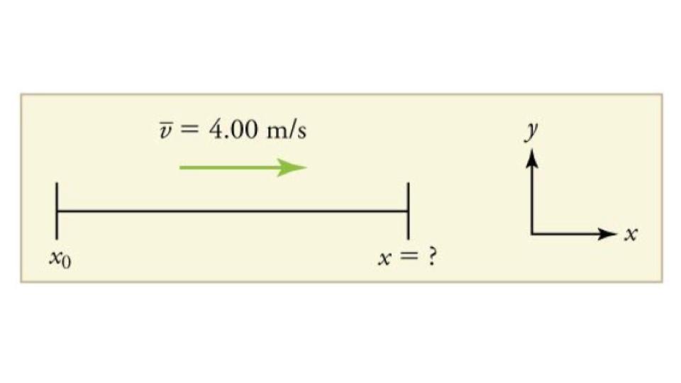
Figure 7.19
The final position x is given by the equation
x = x0+(average v)t.
To find x, we identify the values of x0, and t from the statement of the problem and substitute them into the equation.
Solution
- Identify the knowns. v = 4.00 m/s, Δt = 2.00, and x0 = 0 m.
- Enter the known values into the equation.
x = x0+(average v)t = 0+(4.00 m/s)(120 s) = 480 m
Discussion
Velocity and final displacement are both positive, which means they are in the same direction.
The equation x = x0+(average v)t gives insight into the relationship between displacement, average velocity, and time. It shows, for example, that displacement is a linear function of average velocity. On a car trip, for example, we will get twice as far in a given time if we average 90 km/h than if we average 45 km/h.
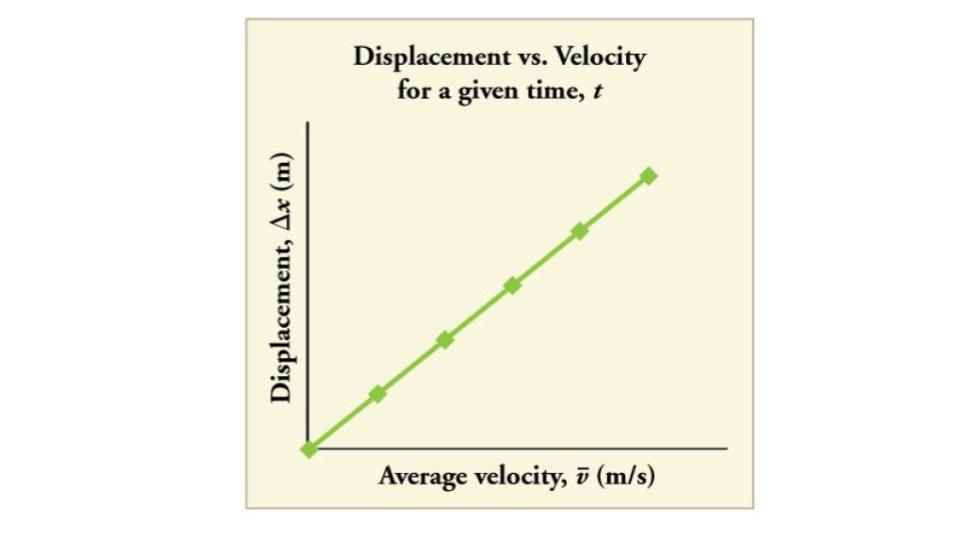
Figure 7.20 There is a linear relationship between displacement and average velocity. For a given time t, an object moving twice as fast as another object will move twice as far as the other object.
SOLVING FOR FINAL VELOCITY
We can derive another useful equation by manipulating the definition of acceleration.
a = Δv/Δt
Substituting the simplified notation for Δv and Δt gives us constant a = (v−v0)/t.
Solving for v yields
v = v0+at (constant a).
EXAMPLE 7.7 CALCULATING FINAL VELOCITY: AN AIRPLANE SLOWING DOWN AFTER LANDING
An airplane lands with an initial velocity of 70.0 m/s and then decelerates at 1.50 m/s2 for 40.0 s. What is its final velocity?
Strategy
Draw a sketch. We draw the acceleration vector in the direction opposite the velocity vector because the plane is decelerating.
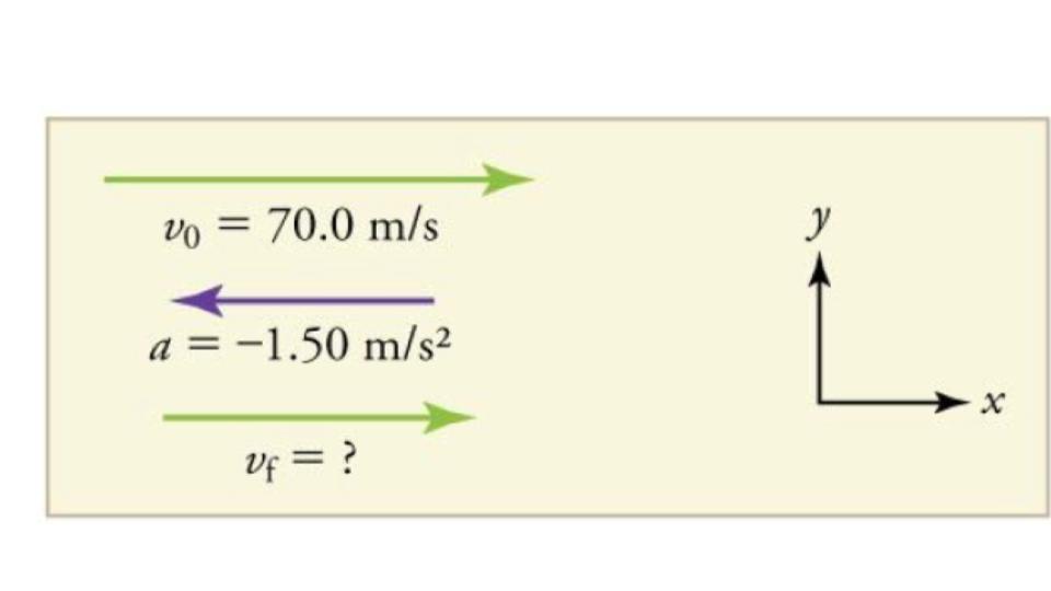
Figure 7.21
Solution
- Identify the knowns. v0 = 70.0 m/s, a = −1.50 m/s2, t = 40.0s
- Identify the unknown. In this case, it is final velocity, vf.
- Determine which equation to use. We can calculate the final velocity using the equation v = v0+at.
- Plug in the known values and solve.
v = v0+at = (70.0 m/s)+(−1.50 m/s2)(40.0 s) = 10.0 m/s
Discussion
The final velocity is much less than the initial velocity, as desired when slowing down, but still positive. With jet engines, reverse thrust could be maintained long enough to stop the plane and start moving it backward. That would be indicated by a negative final velocity, which is not the case here.
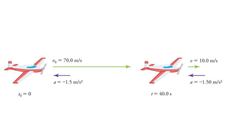
Figure 7.22 The airplane lands with an initial velocity of 70.0 m/s and slows to a final velocity of 10.0 m/s before heading for the terminal. Note that the acceleration is negative because its direction is opposite to its velocity, which is positive.
In addition to being useful in problem solving, the equation v = v0+at gives us insight into the relationships among velocity, acceleration, and time. From it we can see, for example, that
- final velocity depends on how large the acceleration is and how long it lasts
- if the acceleration is zero, then the final velocity equals the initial velocity (v = v0), as expected (i.e., velocity is constant)
- if a is negative, then the final velocity is less than the initial velocity
(All of these observations fit our intuition, and it is always useful to examine basic equations in light of our intuition and experiences to check that they do indeed describe nature accurately.)
MAKING CONNECTIONS: REAL-WORLD CONNECTION
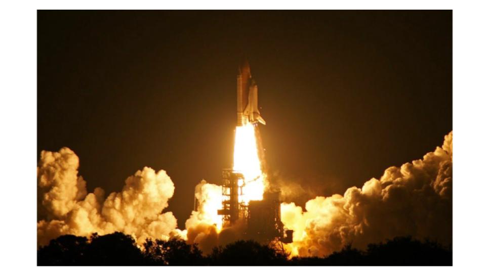
Figure 7.23 The Space Shuttle Endeavor blasts off from the Kennedy Space Center in February 2010. (credit: Matthew Simantov, Flickr)
An intercontinental ballistic missile (ICBM) has a larger average acceleration than the Space Shuttle and achieves a greater velocity in the first minute or two of flight (actual ICBM burn times are classified—short-burn-time missiles are more difficult for an enemy to destroy). But the Space Shuttle obtains a greater final velocity, so that it can orbit the earth rather than come directly back down as an ICBM does. The Space Shuttle does this by accelerating for a longer time.
SOLVING FOR FINAL POSITION WHEN VELOCITY IS NOT CONSTANT (a ≠ 0)
We can combine the equations above to find a third equation that allows us to calculate the final position of an object experiencing constant acceleration. We start with
v = v0+at.
Adding v0 to each side of this equation and dividing by 2 gives
(v0+v)/2 = v0+(1/2)at.
Since (v0+v)/2 = v for constant acceleration, then v = v0+(1/2) at2
Now we substitute this expression for v into the equation for displacement, x = x0+vt, yielding
x = x0+v0t+(1/2)at2 (constant a).
EXAMPLE 7.8 CALCULATING DISPLACEMENT OF AN ACCELERATING OBJECT: DRAGSTERS
Dragsters can achieve average accelerations of 26.0 m/s2. Suppose such a dragster accelerates from rest at this rate for 5.56 s. How far does it travel in this time?
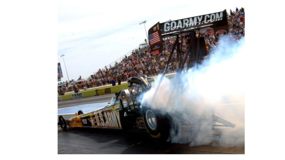
Figure 7.24 U.S. Army Top Fuel pilot Tony “The Sarge” Schumacher begins a race with a controlled burnout. (credit: Lt. Col. William Thurmond. Photo Courtesy of U.S. Army.)
Strategy
Draw a sketch
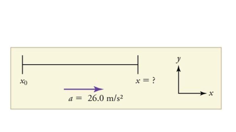
Figure 7.25
We are asked to find displacement, which is x if we take x0 to be zero. (Think about it like the starting line of a race. It can be anywhere, but we call it 0 and measure all other positions relative to it.) We can use the equation x = x0+v0t+(1/2)at2 once we identify v0, and t from the statement of the problem.
Solution
- Identify the knowns. Starting from rest means that v0 = 0, a is given as 26.0 m/s2 is given as 5.56 s.
- Plug the known values into the equation to solve for the unknown x. x = x0+v0t+(1/2)at2
Since the initial position and velocity are both zero, this simplifies to
x = (1/2)at2.
Substituting the identified values of a and t
gives
x = (1/2)(26.0 m/s2)(5.56 s)2,
yielding
x = 402 m.
Discussion
If we convert 402 m to miles, we find that the distance covered is very close to one quarter of a mile, the standard distance for drag racing. So the answer is reasonable. This is an impressive displacement in only 5.56 s, but top-notch dragsters can do a quarter mile in even less time than this.
What else can we learn by examining the equation x = x0+v0t+(1/2)at2 We see that:
- displacement depends on the square of the elapsed time when acceleration is not zero. In Example 7.8, the dragster covers only one fourth of the total distance in the first half of the elapsed time
- if acceleration is zero, then the initial velocity equals average velocity (v0 = v) and x = x0+v0t+(1/2)at2 becomes x = x0+v0t
SOLVING FOR FINAL VELOCITY WHEN VELOCITY IS NOT CONSTANT (a≠0)
A fourth useful equation can be obtained from another algebraic manipulation of previous equations.
If we solve v = v0+at, we get
t = (v−v0)/a.
Substituting this and average v = (v0+v)/2 into x = x0+(average v)t, we get
v2 = v02+2a(x−x0) (constant a).
SUMMARY OF KINEMATIC EQUATIONS (CONSTANT a)
x = x0+(average v)t
average v = (v0+v)/2
v = v0+at
x = x0+v0t+(1/2)at2
v2 = v02+2a(x−x0)
